Driven Kerr resonator
Follow a driven, lossy Kerr resonator from an unstable initial state toward its two metastable branches. We will discover the optimal gauges, compare the trajectory dynamics with a master-equation solution, inspect the Wigner functions, and enable the reduced propagation of Layer III.
Run the code blocks in order in one Julia session, starting from the repository root. See Running the examples for the environment setup.
- Prepare the environment
- Load the packages
- Define the Kerr model
- Discover the stable gauges and choose the initial state
- Compare with trajectory-based gauge discovery
- Evolve the ensemble and a reference solution
- Inspect ensemble and trajectory Wigner functions
- Enable Layer III
Prepare the environment
import Pkg
repo_root = pwd()  # Start Julia from the repository root.
examples_dir = joinpath(repo_root, "examples")
Pkg.activate(examples_dir)
Pkg.develop(Pkg.PackageSpec(path=repo_root))
Pkg.instantiate()
Load the packages
QuantumToolbox supplies the operators and reference solver; DiSLOUTrajectories.jl supplies gauge discovery and trajectory propagation, and CairoMakie draws the figures.
using CairoMakie
using DiSLOUTrajectories
using QuantumToolbox
using Random
Define the Kerr model
The rotating-frame Hamiltonian and physical collapse operator are
\[H=-\Delta a^\dagger a+\frac{K}{2}a^{\dagger 2}a^2 +i(\varepsilon a^\dagger-\varepsilon^*a), \qquad C=\sqrt{\kappa}\,a.\]
Use a Fock cutoff of $N=190$ and the bistable drive $\varepsilon=22.217$. With $\kappa=1$, the time values below also represent $\kappa t$.
N = 190
κ, Δ, K = 1.0, 13.0, 0.2
ε = 22.217 + 0im

a = destroy(N)
n_op = a' * a
# H and C = √κ a (Eq. 7).
H = -Δ * a' * a + (K / 2) * a'^2 * a^2 + im * (ε * a' - conj(ε) * a)
c_ops = [sqrt(κ) * a]
Discover the stable gauges and choose the initial state
Semiclassical discovery solves the mean-field equation of the mode on coherent states of the model operators. limits bounds the occupation searched for fixed points, and keeps their coherent states well inside the Fock cutoff. Stable roots become gauge centers, while any unstable root remains available in the diagnostics.
sc = discover_gauges(
    H, c_ops;
    method=:semiclassical,
    mode_ops=[a],
    mode_dims=[N],
    limits=(120,),
)

α_saddle = only(sc.diagnostics.rejected)
Now construct a coherent initial state at that saddle. This starts the evolution away from either stable center. Store the discovered shifts for the later trajectory solves.
ψ0 = coherent(N, α_saddle)
Z = sc.shifts

(; stable_centers=sc.centers, unstable_saddle=α_saddle)
(stable_centers = ComplexF64[0.0726626169192964 + 1.7953859931208263im 1.741422945981564 - 8.622402989013775im], unstable_saddle = 1.111601973670237 + 6.939543439607221im)The stable centers are near $0.0727+1.7954i$ and $1.7414-8.6224i$. The rejected fixed point near $1.1116+6.9395i$ is the unstable saddle used for the initial coherent state. Z contains collapse-operator shifts $\zeta^{(g)}=-\sqrt{\kappa}\alpha_g$.
Compare with trajectory-based gauge discovery
As a second way to locate the branches, we can evolve 200 preliminary trajectories and cluster their terminal amplitudes. The saved output reports two clusters and three semiclassical fixed points: the latter count includes the unstable saddle.
trajectory_gauges = discover_gauges(H, c_ops;
    method=:trajectories,
    mode_ops=[a],
    mode_dims=[N],
    discovery_time=3.0,
    seed_radii=[sqrt(N - 1)],
    cluster_scales=[1.0],
    step=5.0,
    nseeds=200,
    terminal_window=0.0,
    dbscan_radius=1.5,
    min_neighbors=10,
    min_weight=0.02,
    rng=Xoshiro(1),
)

preflight_positions = vec(trajectory_gauges.diagnostics.terminal_means)
preflight_labels = trajectory_gauges.diagnostics.labels
trajectory_centers = vec(trajectory_gauges.centers)
semiclassical_points = vec(sc.diagnostics.roots)

(; preflight_trajectories=length(preflight_positions),
    trajectory_gauges=length(trajectory_centers),
    semiclassical_solutions=length(semiclassical_points))
(preflight_trajectories = 200, trajectory_gauges = 2, semiclassical_solutions = 3)Plot the preliminary trajectory endpoints, the cluster centers, and all semiclassical fixed points in the complex-amplitude plane.
fig_gauges = Figure(size=(700, 550))
ax_gauges = Axis(fig_gauges[1, 1];
    xlabel="Re⟨a⟩", ylabel="Im⟨a⟩",
    title="Trajectory and semiclassical gauge discovery",
    aspect=DataAspect())

scatter!(ax_gauges, real.(preflight_positions), imag.(preflight_positions);
    color=preflight_labels, colormap=:tab10, markersize=8,
    label="Final preflight positions")
scatter!(ax_gauges, real.(trajectory_centers), imag.(trajectory_centers);
    marker=:circle, markersize=22, color=:transparent,
    strokecolor=:black, strokewidth=2,
    label="Trajectory-deduced gauges")
scatter!(ax_gauges, real.(semiclassical_points), imag.(semiclassical_points);
    marker=:xcross, markersize=20, color=:red, strokewidth=3,
    label="Semiclassical solutions")
axislegend(ax_gauges; position=:lt)
fig_gauges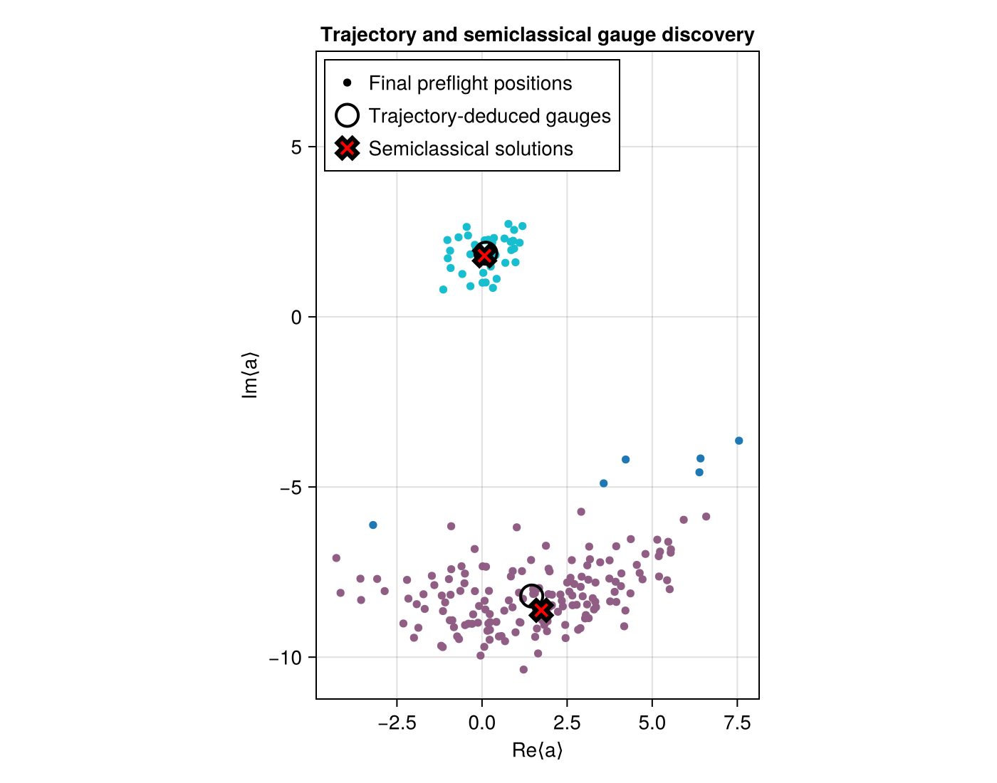
The two endpoint clusters identify the dim and bright branches. Compare their centers with the stable semiclassical roots: finite pilot trajectories and quantum fluctuations need not give exactly the same centers but in this case they are very close.
Evolve the ensemble and a reference solution
First use mesolve for the deterministic master-equation reference, then dislou_solve for 512 trajectories with Layers I and II. Both receive the same physical H, c_ops, initial state, and photon-number observable. Do not shift the physical operators yourself: DiSLOU applies the gauge transformation.
Save the states at three times and keep every trajectory (keep_runs_results), so that we can inspect individual observables and Wigner functions below. The last line counts the quantum jumps of all trajectories.
tlist = collect(range(0.0, 5.0; length=201))
snapshot_times = [0.0, 2.5, 5.0]
ntraj = 512
ensemble_seed = 20260829

mesolve_sol = mesolve(H, ψ0, tlist, c_ops;
    e_ops=[n_op],
    progress_bar=false,
    reltol=1e-8,
    abstol=1e-10,
)

sol = dislou_solve(H, ψ0, tlist, c_ops;
    e_ops=[n_op],
    gauge_set=Z,
    ntraj=ntraj,
    rng=Xoshiro(ensemble_seed),
    saveat=snapshot_times,
    keep_runs_results=Val(true),
)
sum(length, sol.col_times)38946Read the photon-number dynamics
average_expect(sol) averages the trajectories, and std_expect(sol) gives their standard deviation; divided by $\sqrt{N_{\rm traj}}$ it is the standard error of the mean. Plot the photon number against mesolve, then show six individual trajectories, sol.expect[1, trajectory, :], below. The shaded band describes the uncertainty of the ensemble mean.
n_mean = real.(average_expect(sol)[1, :])
n_sem = std_expect(sol)[1, :] ./ sqrt(ntraj)
n_mesolve = real.(mesolve_sol.expect[1, :])
selected_trajectories = 1:6

fig_n = Figure(size=(900, 700))
ax_mean = Axis(fig_n[1, 1]; xlabel="κt", ylabel="⟨a†a⟩",
    title="Ensemble photon number and master-equation reference")
band!(ax_mean, tlist, n_mean .- n_sem, n_mean .+ n_sem;
    color=(:steelblue, 0.25), label="DiSLOU standard error")
lines!(ax_mean, tlist, n_mean;
    color=:steelblue, linewidth=2, label="DiSLOU mean")
lines!(ax_mean, tlist, n_mesolve;
    color=:black, linestyle=:dash, linewidth=2, label="mesolve")
axislegend(ax_mean; position=:lt)

ax_traj = Axis(fig_n[2, 1]; xlabel="κt", ylabel="⟨a†a⟩",
    title="Six individual trajectories")
for trajectory in selected_trajectories
    lines!(ax_traj, tlist, real.(sol.expect[1, trajectory, :]);
        label="trajectory $trajectory")
end
axislegend(ax_traj; position=:rt, nbanks=2)
fig_n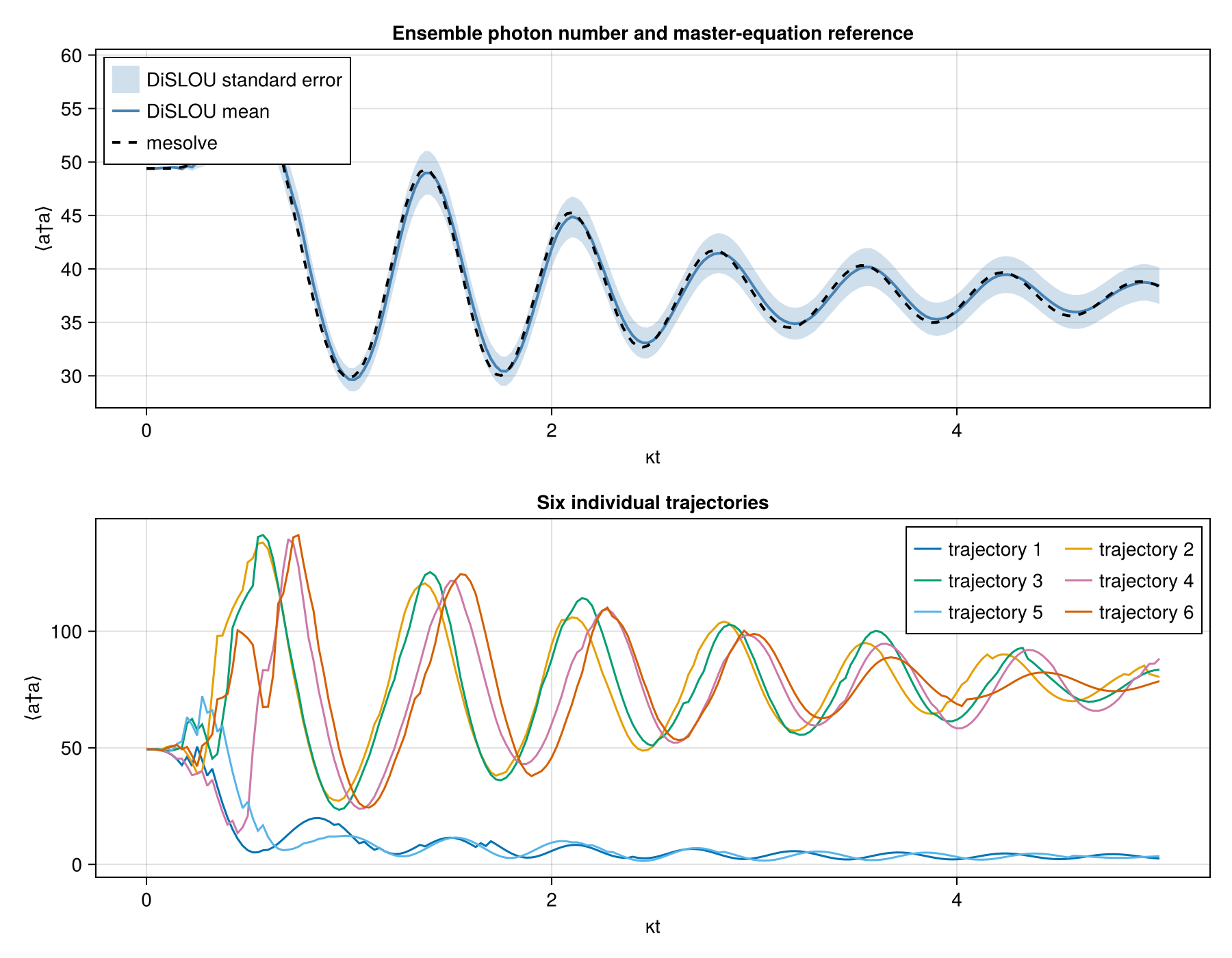
The ensemble follows the oscillatory relaxation of the master-equation reference, while individual trajectories separate toward the two branches, clearly showing the bistable nature of the model.
Inspect ensemble and trajectory Wigner functions
At the final saved time, compare the reconstructed ensemble state with trajectories 1–3. These are different views of the same simulation: the ensemble combines all trajectories, while each other panel shows one conditional state.
xvec = collect(range(-10.0, 10.0; length=201))
yvec = collect(range(-15.0, 5.0; length=201))
time_index = length(snapshot_times)
scaled_snapshot_time = κ * snapshot_times[time_index]

wigner_states = (
    average_states(sol)[time_index],
    sol.states[1, time_index],
    sol.states[2, time_index],
    sol.states[3, time_index],
)
wigner_values = map(
    state -> wigner(state, xvec, yvec),
    wigner_states,
)

wigner_plots = transpose.(wigner_values)
for W in wigner_plots
    @assert size(W) == (length(xvec), length(yvec))
    peak = Tuple(argmax(abs.(W)))
    # @assert 1 < peak[1] < length(xvec)
    # @assert 1 < peak[2] < length(yvec)
end

color_limit = maximum(maximum(abs, W) for W in wigner_values)
panel_positions = ((1, 1), (1, 2), (2, 1), (2, 2))
panel_titles = (
    "Ensemble at κt = $scaled_snapshot_time",
    "Trajectory 1 at κt = $scaled_snapshot_time",
    "Trajectory 2 at κt = $scaled_snapshot_time",
    "Trajectory 3 at κt = $scaled_snapshot_time",
)

fig_w = Figure(size=(600, 500))
heatmaps = Any[]
for (position, title, W) in zip(panel_positions, panel_titles, wigner_plots)
    row, column = position
    ax = Axis(fig_w[row, column];
        xlabel="x", ylabel="y", title, aspect=DataAspect())
    push!(heatmaps, heatmap!(ax, xvec, yvec, W;
        colormap=:balance, colorrange=(-color_limit, color_limit)))
end
Colorbar(fig_w[:, 3], first(heatmaps); label="W(x, y)")
fig_w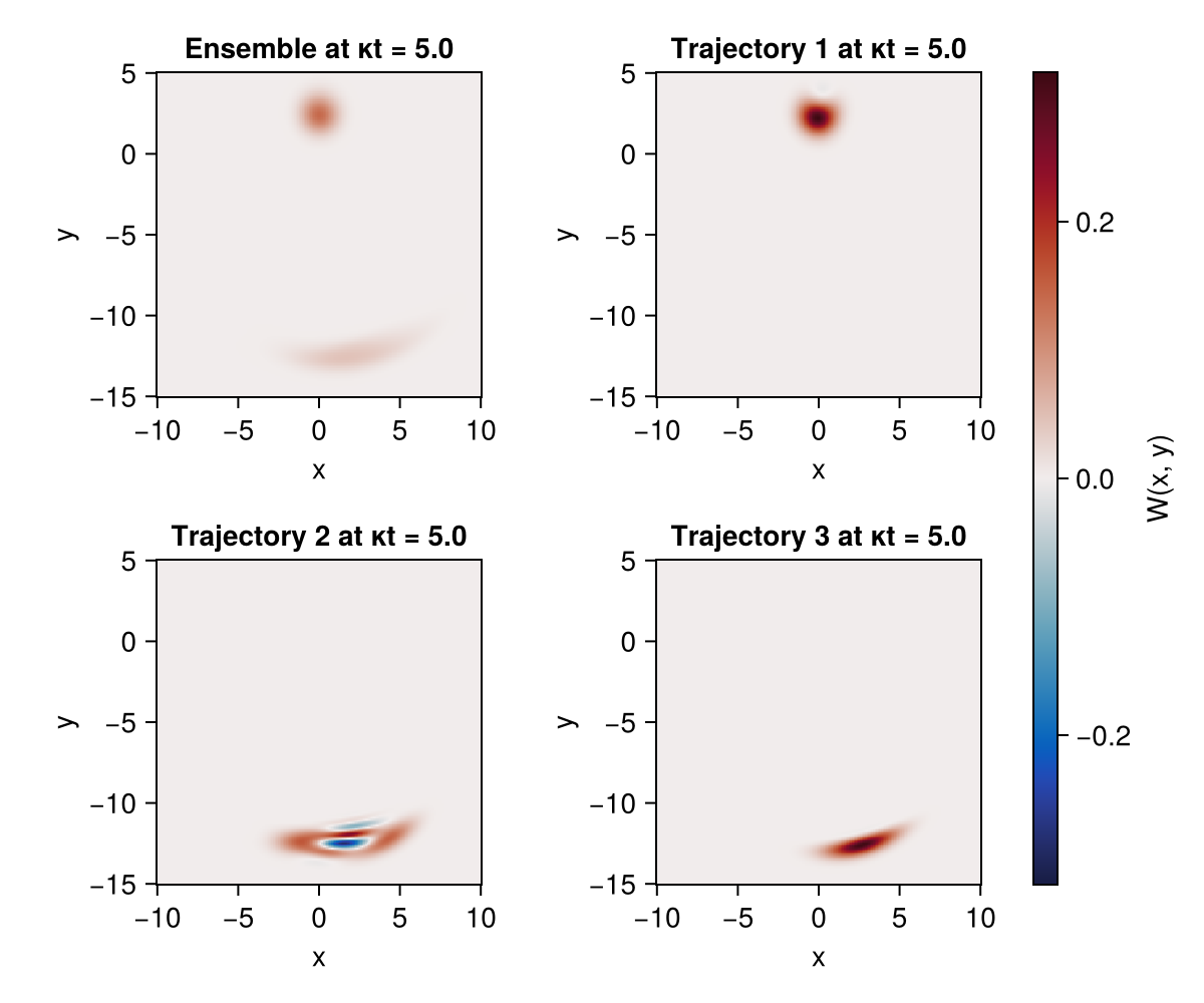
The ensemble panel contains contributions from both branches. while the three individual panels show which region each selected trajectory occupies at the final time: they are all close to one of the metastable states.
Enable Layer III
Repeat the solve with the same state, gauges, trajectory count, and seed, adding the reduced-space options. The entries of layer3_sizes follow the gauge columns: $m^{(-)}=20$ for the dim branch and $m^{(+)}=60$ for the bright branch.
The residual tolerance $r_{\rm tol}=10^{-4}$ controls acceptance of a projection into a reduced space, as in Eq. (21). The solver falls back to the full basis when the projection residual goes above it.
layer3_sol = dislou_solve(H, ψ0, tlist, c_ops;
    e_ops=[n_op],
    gauge_set=Z,
    ntraj=ntraj,
    rng=Xoshiro(ensemble_seed),
    layer3_sizes=[20, 60],
    residual_tolerance=1e-4,
    keep_runs_results=Val(true),
)
sum(length, layer3_sol.col_times)38946Overlay the Layer III result with Layers I and II and mesolve, keeping the standard-error bands for both ensembles.
n_layer3 = real.(average_expect(layer3_sol)[1, :])
n_layer3_sem = std_expect(layer3_sol)[1, :] ./ sqrt(ntraj)

fig_validation = Figure(size=(900, 450))
ax_validation = Axis(fig_validation[1, 1];
    xlabel="κt", ylabel="⟨a†a⟩",
    title="Layers I + II, Layer III, and mesolve")
band!(ax_validation, tlist, n_mean .- n_sem, n_mean .+ n_sem;
    color=(:steelblue, 0.18))
band!(ax_validation, tlist,
    n_layer3 .- n_layer3_sem, n_layer3 .+ n_layer3_sem;
    color=(:darkorange, 0.18))
lines!(ax_validation, tlist, n_mean;
    color=:steelblue, linewidth=2, label="Layers I + II")
lines!(ax_validation, tlist, n_layer3;
    color=:darkorange, linewidth=2, label="Layer III")
lines!(ax_validation, tlist, n_mesolve;
    color=:black, linestyle=:dash, linewidth=2, label="mesolve")
axislegend(ax_validation; position=:lt)
fig_validation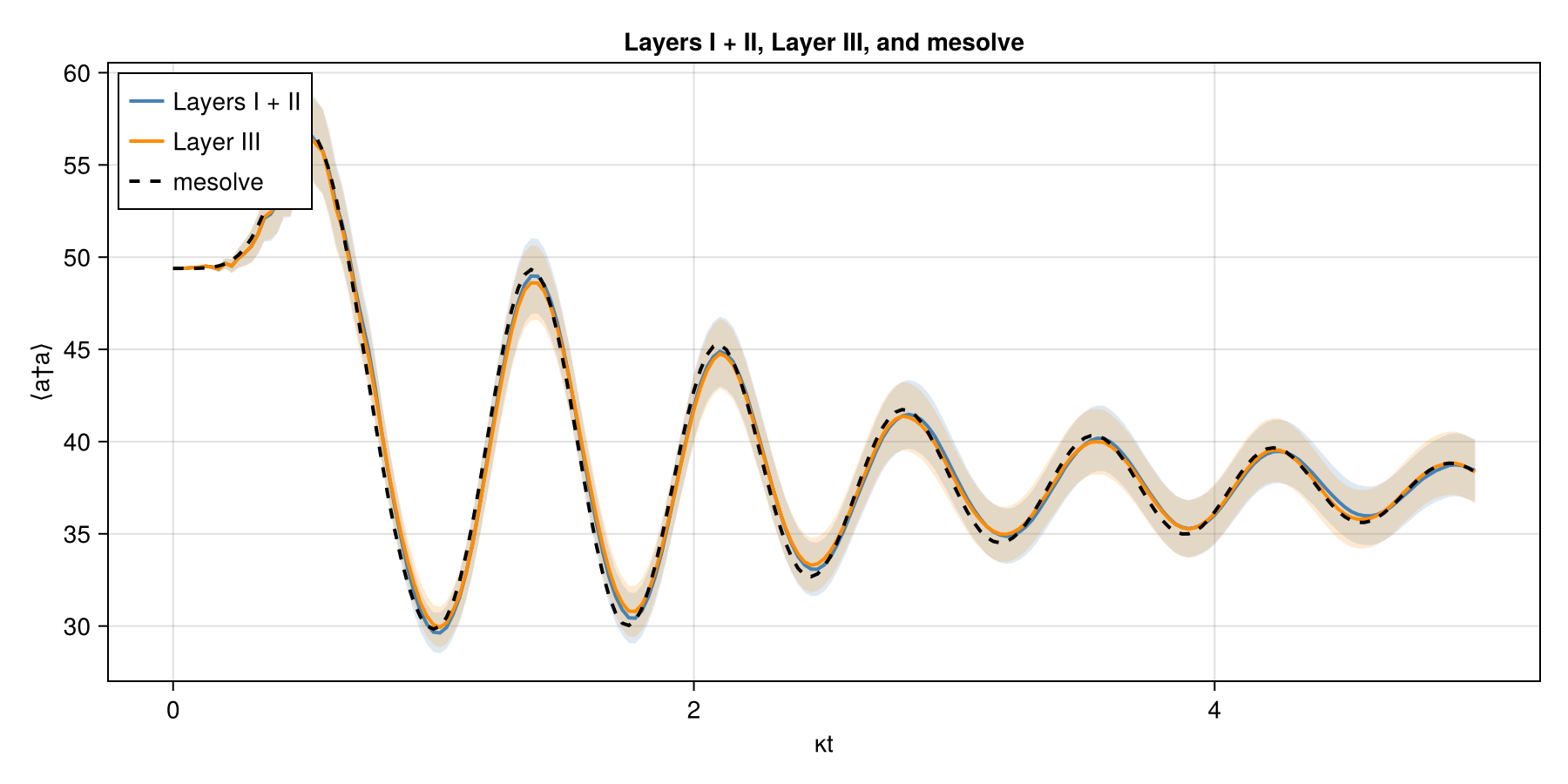
The comparison confirms that the reduced and full-space ensemble curves track the same reference dynamics.
Continue with the two-mode ideal cat to apply the same workflow to multiple modes and jump operators.